Recently at work I spent some time trying to optimize large sparse matrix multiplication on Hadoop as part of an implementation of a larger algorithm (Markov Clustering). We ended up pursuing a different route, but I decided to continue pursuing the problem on my own time. I learned a fair amount, and I don’t think there exists a much better way of doing this out there. So I decided to write up an explanation of the algorithms involved, as well as release the code:
https://github.com/jfkelley/hadoop-matrix-mult
This post assumes knowledge of Hadoop, or at least the MapReduce paradigm, as well as the mathematical definition of matrix multiplication.
The problem I was faced with was to multiply two large square matrixes. Each one roughly 500,000 x 500,000. The only good news was that both were relatively sparse: about 1 billion non-zero entries, or roughly 0.4% of all possible entries. The algorithms I’ll discuss apply to larger or smaller matrixes, but I’ll use these as a point of reference for discussion.
Throughout this post, I’ll refer to the matrixes in the multiplication as \(AB=C\), with elements \(a_{ij}\), \(b_{ij}\), and \(c_{ij}\) such that \(c_{ij}=\sum_{k=1}^n{a_{ik}b_{kj}}\).
The most basic matrix multiplication algorithm is pretty straight-forward to implement based on that formula:
public static double[][] multiply(double[][] a, double[][] b) {
	assert(a[0].length == b.length);
	double[][] c = new double[a.length][b[0].length];
	for (int i = 0; i < c.length; i++) {
		for (int j = 0; j < c[i].length; j++) {
			double sum = 0.0;
			for (int k = 0; k < a[0].length; k++) {
				sum += a[i][k] * b[k][j];
			}
			c[i][j] = sum;
		}
	}
	return c;
}
However, there are several obvious problems:
- These matrixes are way too big to fit in memory at once. This code requires three 2-d arrays of doubles, each 500k x 500k. 500k * 500k * 3 * 8 bytes = 6 TB
- This is not distributed at all. This is a lot of computation - O(n^3) - so I’d like to take advantage of all the hundreds or thousands of cores in my Hadoop cluster
- There’s no taking advantage of the sparsity of the matrixes. There will be a lot of
sum += 0.0 * 0.0being executed, which is wasteful.
So I decided to tackle the non-distributed problem first. Whenever you’ve got a big data algorithm problem, a great text to start with is Mining Massive Datasets by Leskovec, Rajaraman, and Ullman. It’s available for free online at http://www.mmds.org. I very highly recommend it.
Sure enough, the book proposes two different algorithms. The first is based on the fact that if you store the matrixes as a tuples (i, j, x) meaning \(a_{ij}=x\), then the multiplication is equivalent to a relation algebra join followed by a group by and aggregation. In SQL terms, it’s:
SELECT A.i, B.j, SUM(A.x * B.x)
FROM A join B on A.j = B.i
GROUP BY A.i, B.j
Both the join and aggregation operations have relatively straightforward implementations in MapReduce. Here’s the join in pseudo-code:
map(i, j, x, isLeft):
	if (isLeft):
		emit(j, (i, j, x, isLeft))
	else:
		emit(i, (i, j, x, isLeft))

reduce(k, elements):
	left = filter elements where element.isLeft
	right = filter elements where !element.isLeft
	for (i1, j1, x1) in left:
		for (i2, j2, x2) in right:
			emit (i1, j2, x1 * x2)
And the aggregation is even easier:
map(i, j, x):
	emit((i, j), x)

reduce((i, j), xs):
	emit (i, j, sum(xs))
This algorithm has one major flaw, though. The intermediate data between the two jobs is explosively large. If a typical row/column has \(k\) non-zero entries, then \(k^2\) records are emitted in each call to reduce in the first job. Since the matrixes I was aiming to handle have on average 2000 entries per row, this results in a 2000x increase in data volume. What was originally a manageable 16 GB is suddenly a pretty unwieldy 32 TB. Of course, that would be decreased back down after the aggregation phase, but it’s still very slow to generate and write out all of that data.
The second algorithm suggested in MMDS is based on the idea that the reduce key should be the index of the resulting output value. So we should set the reduce key to be (i,j) for all values needed to calculate \(c_{ij}\). What values are needed? \(a_{i1}, a_{i2}, a_{i3}... a_{in}\) as well as \(b_{1j}, b_{2j}, b_{3j}... b_{nj}\). But to actually come up with the map function, it’s easier to consider the reverse question: which output values is \(a_{ij}\) used in the calculation of? That would be \(c_{i1}, c_{i2}, c_{i3}... c_{in}\). For \(b_{ij}\) it’s \(c_{1j}, c_{2j}, c_{3j}... c_{nj}\). From that it’s natural to translate into this pseudo-code:
map(i, j, x, isLeft):
	if (isLeft):
		for k in 1 to n:
			emit((i, k), (i, j, x, isLeft))
	else:
		for k in 1 to n:
			emit((k, j), (i, j, x, isLeft))

reduce((i, j), elements):
	left = filter elements where element.isLeft
	right = filter elements where !element.isLeft
	paired = align left, right based on left.col == right.row
	sum = 0
	for (i1, j1, x1), (i2, j2, x2) in paired:
		sum += x1 * x2
	emit(i, j, sum)
This has the benefit of only requiring one MapReduce job, but the data volume between the map and reduce phases (in the shuffle-sort) is even worse than before. In this case, that data is 500,000x as large!
So the book wasn’t that helpful, but it did set me down the right sort of path. The algorithm I settled on is based on submatrix multiplication. I split both input matrixes into a configurable number of submatrixes (call it \(s\)), and the reduce key corresponds to the multiplication of two submatrixes. After the submatrix multiplication, there’s another MapReduce job that simply does the same aggregation as before, except with this version the intermediate data is only \(s\) times as large.
map(i, j, x, isLeft):
	(sub_i, sub_j) = submatrix_membership(i, j, s)
	for k in 1 to s:
		if (isLeft):
			emit((sub_i, sub_j, k), (i, j, x, isLeft))
		else:
			emit((k, sub_i, sub_j), (i, j, x, isLeft))

reduce((sub_i, sub_k, sub_j), elements):
	left = filter elements where element.isLeft
	right = filter elements where !element.isLeft
	left_submatrix = as_matrix(left)
	right_submatrix = as_matrix(right)
	result = left_submatrix * right_submatrix // standard in-memory matrix multiply
	for (i, j, x) in result:
		emit(i, j, x)

map(i, j, x):
	emit((i, j), x)

reduce((i, j), xs):
	emit (i, j, sum(xs))
Here’s are summary statistics of each part of the job that hopefully explains why this is a much more efficient algorithm:
- Total input non-zero elements
\(= N\) - Submatrix splits (in each dimension)
\(= s\) - Map-1 output records = Reduce-1 input records
\(= Ns\) - Reduce-1 number of keys
\(= s^3\) - Reduce-1 records per key
\(= \frac{N}{s^2}\) - Reduce-1 output data volume = Map-2 input data volume
\(\propto Ns\) - Reduce-2 output data volume
\(\propto N\)
Here the multiplication in data volume is \(s\), but that can be set fairly low. There are two requirements: first, the number of reduce keys \(s^3\) must be enough to “saturate” the reduce slots on the cluster. It should be roughly the total number of cores, or perhaps 2 or 3 times more, to avoid potential skew. Second, a single reduce task must be able to hold \(\frac{N}{s^2}\) elements in memory and execute the submatrix multiplication. The good news is that this means as the data volume grows, the “multiplication factor” grows sub-linearly: O(N^1⁄2). In practice, \(10 \leq s \leq 50\) is a reasonable expectation.
There’s some additional optimization that can be done as well. The second job can make use of a combiner that is the same as the reducer. Furthermore, a custom partitioner can be used in the first job so that submatrix multiplications that will contribute to the same final output value happen in the same reduce task. Thus those output values will be part of the same file, and then part of the same map task in the second job, so the combiner will be more effective. In fact, it’s also possible to push this “combining” logic back into the first reduce phase, at the cost of some extra memory.
The remaining piece of the puzzle is the submatrix multiplication. I wanted to avoid reinventing the wheel if possible, so I began looking for Java matrix libraries. I found about 40 of them. However, none that I could find met four basic requirements I had:
- Decipherable documentation or at least some mention of their popular use
- Sparse matrix storage
- Matrix multiplication utilizing sparsity
- Matrix multiplication outputting into sparse storage
The last two discounted a lot of libraries. Fair enough, I decided to implement my own. I thought, “How hard could it be?”
My first attempt was to store each non-zero element in a map from its coordinates to it’s value, with missing elements implicitly 0. I used a HashMap <IntPair, Double>. Additionally, to make multiplication feasible, the left matrix needs a map from each row index to the column indexes containing non-zero elements in that row. And the right matrix needs the transpose: a map from each column index to the row indexes containing non-zero elements in that column: a HashMap <Integer, TreeSet <Integer>>.
So, I implemented this without too much trouble, and went to compare its running time and memory usage against two popular libraries (that both failed one of the above requirements): JBLAS and Colt. The results were pretty terrible.
First of all, there’s a lot of memory bloat and overhead involved. An IntPair class has some overhead just because it’s a Java class, as does a Double (not a double). TreeSet also has tons of overhead. I could certainly use something else there, but memory wasn’t the biggest problem…
The run time was at least 100x slower than either Colt or JBLAS. I think the main reason is probably the memory access pattern. When accessing values out of a HashMap or a TreeSet, the sequence of memory accesses is pretty much random. There are lots of little objects all over the heap. And even where they’re somewhat consolidated (the HashMap’s main array), the positions within that chunk are accessed in random order. With all that in mind, the hardware’s caches are basically no help. And keep in mind the relevant numbers every programmer should know: an L1 cache reference is 100x faster than a main memory reference. And an L2 cache reference is 25x faster. So it definitely does matter. Furthermore, this “random” behavior means that branch prediction is basically no help at all.
So I did some research and found a method called compressed row storage (CRS). It’s used in several of the libraries mentioned earlier, but not quite in the way I wanted.
In CRS, you store three things
- A large array of doubles (“values”) containing only the non-zero elements of the array, in row-major order.
- An equally large array of integers (“col_indexes”) containing the column-indexes of the corresponding elements in the double array
- A smaller array of integers (“row_pointers”) containing the locations in the two large arrays where new rows start.
As an example, consider this matrix:
In CRS, it would be stored as:
values:       [2, 3, 5, 1, 2, 1, 1]
col_indexes:  [1, 3, 0, 1, 3, 1, 2]
row_pointers: [0, 2, 4, 5]
You can also do the transpose - compressed column storage - which is very similar. The values are stored in column-major order, row indexes are stored instead of column indexes, and start-of-column pointers are stored instead of start-of-row pointers. The above matrix as CCS would be:
values:       [5, 2, 1, 1, 1, 3, 2]
row_indexes:  [1, 0, 1, 3, 3, 0, 2]
col_pointers: [0, 1, 4, 5]
Memory-wise, this is about as efficient as it gets. It is 12 bytes (1 double, 1 int) per element, and 4 bytes per row (or per column).
This also enables an extremely fast multiplication, if the left matrix (\(A\)) is stored as CRS, and the right matrix (\(B\)) as CCS. When computing an output value \(c_{ij}\), you need row \(i\) from \(A\) and column \(j\) from \(B\). The row_pointers/col_pointers arrays can be used to find where that row and that column begin and end within the values arrays. Then iterate through just those sections of the arrays and multiply elements with matching values in the col_indexes/row_indexes arrays.
public static void mult(CompRowMatrix a, CompColMatrix b) {
	for (int i = 0; i < a.nRows; i++) {
		for (int j = 0; j < b.nCols; j++) {
			double sum = 0.0;
			int i1 = a.rowPtr[i];
			int i2 = b.colPtr[j];
			int end1 = a.rowPtr[i+1];
			int end2 = b.colPtr[j+1];
			while (i1 < end1 && i2 < end2) {
				if (a.colInd[i1] == b.rowInd[i2]) {
					sum += a.vals[i1++] * b.vals[i2++];
				} else if (a.colInd[i1] < b.rowInd[i2]) {
					i1++;
				} else {
					i2++;
				}
			}
			if (sum != 0.0) {
				emit(i, j, sum);
			}
		}
	}
}
This has a few major benefits. First of all, note that the line sum += a.vals[i1++] * b.vals[i2++] only ever multiplies and adds non-zero values (as only non-zero values are stored). So there is no extraneous arithmetic.
But perhaps the real performance win is that the memory access pattern is great. These large arrays are walked in order. In fact, the entirety of the right matrix’s values array is iterated through in order over and over. The left matrix is accessed in chunks. Perhaps a picture explains it best:
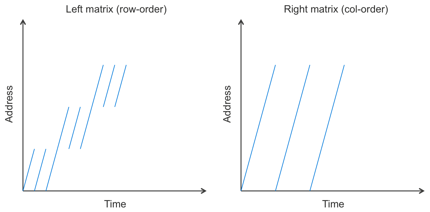
Basically, this means that caching is super-effective. Lots of cache hits, few misses.
Furthermore, branch prediction does pretty well on the inner-most if-elseif-else statement on real-world matrixes. If the matrix were truly random, it would not, but most matrixes are not random. If there’s any structure to which regions of the matrix are non-zero, then branch prediction does much better. There will often be long runs where the same one of those branches is executed over and over.
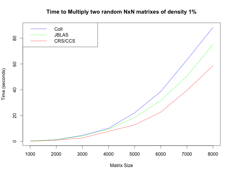
Anyway, I’m happy to say that this implementation actually beats Colt and JBLAS! I ran some really simple benchmarks on my laptop. First, I tested multiplying two random square matrixes of varying size but constant sparsity: 1% non-zero entries:
I also tested it on a constant size but varying sparsity:

You can see here that JBLAS actually does not use an implementation that utilizes the sparsity of the matrix, so that has no effect on its running time. Also note that the crossover point is at about 1%, which is lower than I had expected, but still safely above the 0.4% of the actual matrixes in question.
As a future improvement, I’d like to investigate matrix multiplication methods with better asymptotic performance such as the Strassen algorithm or Coppersmith-Winograd algorithm. I expect there might be a tradeoff between the supposed algorithmic big-O speed up, and the practical details (like caches and branch prediction). It would also be interesting to see if these could be incorporated at the MR level instead of at the submatrix multiplication level.
Remember that my actual implementation is available at https://github.com/jfkelley/hadoop-matrix-mult so if you want to actually use this, go ahead. And there are also a few more notes in the README there about implementation details.